환경 세팅은 해당 사이트를 참고하였습니다.
1. 문제
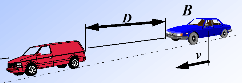
(1) Define the inputs and outputs. There are two inputs : D, the distance between the cars, and v, the velocity of the following car. There is one output: B, the amount of braking to apply to the followin car(force). The inputs and outputs are shown in the figure below.
(2) Define the subsets’ intervals. To simplify things, 3 subsetintervals will be chosen for each variable. These are low, medium and high for distance and velocity, and small, medium and big for braking force.
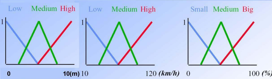
(3) Choose the membership functions. In this example, the shape of the membership functions are fairly simple, just a linear transition between the various subsets (see above figure). To illustrate, the membership function for low distance goes down linearly from 1 to 0 as distance goes from 0 to 5 meters.

(4) Set the IF-THEN rules. This is how combinations of the input determine the output. For example, IF D is low AND v is high, THEN B is big. Similarly, the other rules are defined. This is where the non-quantitative human reasoning comes in. A simple two-rule system could be like that.
(5) Perform calculations and adjust the rules. Since the rules are non-exact some adjustments may be necessary to more optimally control the vehicles' distance.
(Question) If D is 4 meters and v is 70km/hr what percentage braking will be aplied?
2. 코드
import skfuzzy as fuzz
import matplotlib.pyplot as plt
# 범위 설정
x_dist = np.arange(0, 11, 1)
x_vel = np.arange(0, 121, 1)
x_f = np.arange(0, 101, 1)
# 입출력 설정. membeship function 설정
dist_lo = fuzz.trimf(x_dist, [0, 0, 5])
dist_md = fuzz.trimf(x_dist, [0, 5, 10])
dist_hi = fuzz.trimf(x_dist, [5, 10, 10])
vel_lo = fuzz.trimf(x_vel, [0, 0, 60])
vel_md = fuzz.trimf(x_vel, [0, 60, 120])
vel_hi = fuzz.trimf(x_vel, [60, 120, 120])
f_sm = fuzz.trimf(x_f, [0, 0, 50])
f_md = fuzz.trimf(x_f, [0, 50, 100])
f_bg = fuzz.trimf(x_f, [50, 100, 100])
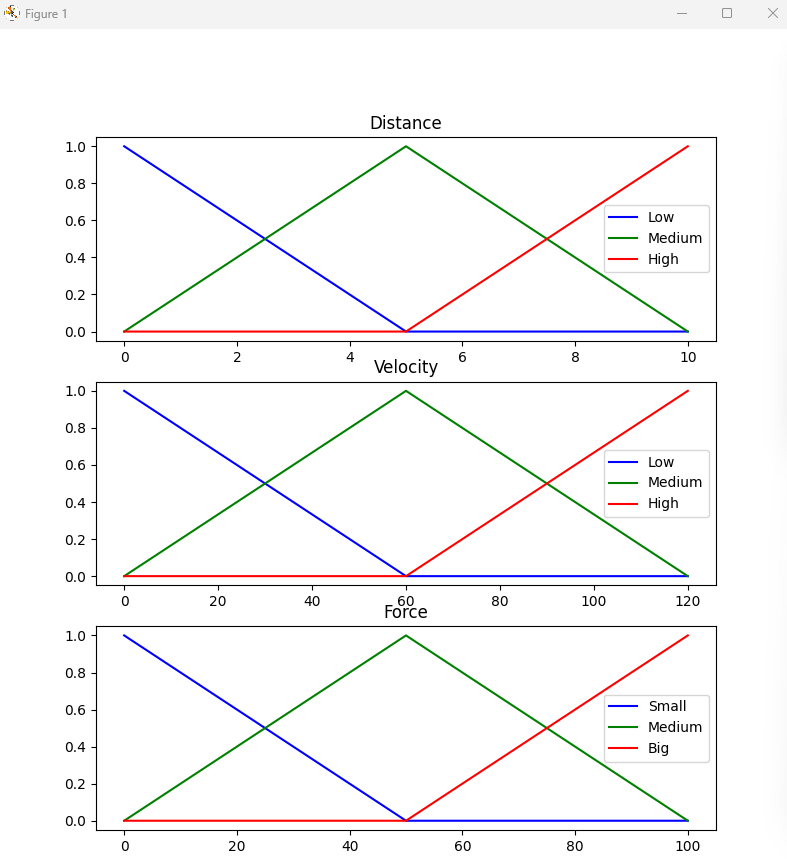
fig, (ax0, ax1, ax2) = plt.subplots(nrows=3, figsize=(8,9))
ax0.plot(x_dist, dist_lo, 'b', linewidth=1.5, label='Low')
ax0.plot(x_dist, dist_md, 'g', linewidth=1.5, label='Medium')
ax0.plot(x_dist, dist_hi, 'r', linewidth=1.5, label='High')
ax0.set_title('Distance')
ax0.legend()
ax1.plot(x_vel, vel_lo, 'b', linewidth=1.5, label='Low')
ax1.plot(x_vel, vel_md, 'g', linewidth=1.5, label='Medium')
ax1.plot(x_vel, vel_hi, 'r', linewidth=1.5, label='High')
ax1.set_title('Velocity')
ax1.legend()
ax2.plot(x_f, f_sm, 'b', linewidth=1.5, label='Small')
ax2.plot(x_f, f_md, 'g', linewidth=1.5, label='Medium')
ax2.plot(x_f, f_bg, 'r', linewidth=1.5, label='Big')
ax2.set_title('Force')
ax2.legend()
# Rule application
dist_level_lo = fuzz.interp_membership(x_dist, dist_lo, 4)
dist_level_md = fuzz.interp_membership(x_dist, dist_md, 4)
dist_level_hi = fuzz.interp_membership(x_dist, dist_hi, 4)
vel_level_lo = fuzz.interp_membership(x_vel, vel_lo, 70)
vel_level_md = fuzz.interp_membership(x_vel, vel_md, 70)
vel_level_hi = fuzz.interp_membership(x_vel, vel_hi, 70)
# RULE 1
active_rule1 = np.fmin(dist_level_lo, vel_level_hi)
f_activation_bg = np.fmin(active_rule1, f_bg)
# RULE 2
active_rule2 = np.fmin(dist_level_md, vel_level_hi)
f_activation_md = np.fmin(active_rule1, f_md)
f0 = np.zeros_like(x_f)
# vis
fig, ax0 = plt.subplots(figsize=(8,3))
#ax0.fill_between(x_f, f0, f_activation_sm, facecolor='b', alpha=0.7)
#ax0.plot(x_f, f_sm, 'b', linewidth = 0.5, linestyle='--', )
ax0.fill_between(x_f, f0, f_activation_md, facecolor='g', alpha=0.7)
ax0.plot(x_f, f_md, 'g', linewidth = 0.5, linestyle='--', )
ax0.fill_between(x_f, f0, f_activation_bg, facecolor='r', alpha=0.7)
ax0.plot(x_f, f_bg, 'r', linewidth = 0.5, linestyle='--', )
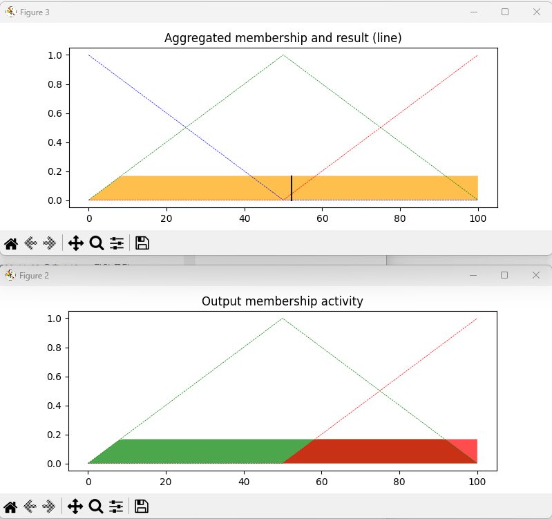
ax0.set_title('Output membership activity')
aggregated = np.fmax(f_activation_md, f_activation_bg)
f = fuzz.defuzz(x_f, aggregated, 'centroid')
f_activation = fuzz.interp_membership(x_f, aggregated, f)
fig, ax0 = plt.subplots(figsize=(8, 3))
ax0.plot(x_f, f_sm, 'b', linewidth = 0.5, linestyle='--', )
ax0.plot(x_f, f_md, 'g', linewidth = 0.5, linestyle='--')
ax0.plot(x_f, f_bg, 'r', linewidth = 0.5, linestyle='--')
ax0.fill_between(x_f, f0, aggregated, facecolor='Orange', alpha=0.7)
ax0.plot([f, f], [0, f_activation], 'k', linewidth=1.5, alpha=0.9)
ax0.set_title('Aggregated membership and result (line)')
plt.show()
(1) 코드 실행 전에, Pycharm 터미널 창에서 다음 라이브러리들을 설치한다.
pip install numpy
pip install matplotlib
pip install -U scikit-fuzzy
(2) 코드 설명 :
코드 설명할 예정입니다 ~~
3. 실행 화면
설명
'LAB > 지능 제어' 카테고리의 다른 글
| 지능제어(1) Introduction (0) | 2023.08.02 |
|---|---|
| 지능제어(2) 임시 (0) | 2023.07.26 |
| 지능제어(2-1) Homework code1 - Truck Backer-Upper Control (0) | 2023.07.26 |


